Last updated: 2020-01-15

Checks: 7 0

Knit directory: Simon_et_al_2020/

This reproducible R Markdown analysis was created with workflowr (version 1.6.0). The Checks tab describes the reproducibility checks that were applied when the results were created. The Past versions tab lists the development history.

R Markdown file: up-to-date

Great! Since the R Markdown file has been committed to the Git repository, you know the exact version of the code that produced these results.

Environment: empty

Great job! The global environment was empty. Objects defined in the global environment can affect the analysis in your R Markdown file in unknown ways. For reproduciblity it’s best to always run the code in an empty environment.

Seed: set.seed(20200113)

The command set.seed(20200113) was run prior to running the code in the R Markdown file. Setting a seed ensures that any results that rely on randomness, e.g. subsampling or permutations, are reproducible.

Session information: recorded

Great job! Recording the operating system, R version, and package versions is critical for reproducibility.

Cache: none

Nice! There were no cached chunks for this analysis, so you can be confident that you successfully produced the results during this run.

File paths: relative

Great job! Using relative paths to the files within your workflowr project makes it easier to run your code on other machines.

Repository version: 389248d

Great! You are using Git for version control. Tracking code development and connecting the code version to the results is critical for reproducibility. The version displayed above was the version of the Git repository at the time these results were generated.

Note that you need to be careful to ensure that all relevant files for the analysis have been committed to Git prior to generating the results (you can use wflow_publish or wflow_git_commit). workflowr only checks the R Markdown file, but you know if there are other scripts or data files that it depends on. Below is the status of the Git repository when the results were generated:


Ignored files:
    Ignored:    .DS_Store
    Ignored:    .Rhistory
    Ignored:    .Rproj.user/
    Ignored:    analysis/.Rhistory
    Ignored:    code/.Rhistory
    Ignored:    data/.DS_Store
    Ignored:    output/.DS_Store
    Ignored:    output/.Rhistory

Untracked files:
    Untracked:  data/RNA/
    Untracked:  data/TCR/
    Untracked:  data/clinical-data/
    Untracked:  data/gene-sets/
    Untracked:  misc/
    Untracked:  output/2019-02-22_RNA-seq_DE_1.RData
    Untracked:  output/2019-02-22_RNA-seq_DE_2.RData
    Untracked:  output/2019-02-22_RNA-seq_DE_3.RData
    Untracked:  output/2019-02-27_TCR-seq_QC.RData
    Untracked:  output/2019-02-28_TCR-seq_EDA.RData
    Untracked:  output/2020-01-12_TCR-seq_EDA_2.RData
    Untracked:  output/RNA_count.rds
    Untracked:  output/RNA_raw_count.rds
    Untracked:  output/TCR_count.rds
    Untracked:  output/TCR_pData.rds
    Untracked:  output/output_2019-02-22/

Note that any generated files, e.g. HTML, png, CSS, etc., are not included in this status report because it is ok for generated content to have uncommitted changes.

These are the previous versions of the R Markdown and HTML files. If you’ve configured a remote Git repository (see ?wflow_git_remote), click on the hyperlinks in the table below to view them.

File	Version	Author	Date	Message
Rmd	389248d	ValentinVoillet	2020-01-15	Edits .Rmd (RNA-seq_DE_3)

File creation: February, 22nd 2019
Update: January, 15th 2020

1 Statistical Analysis

1.1 Differential analysis btw outcomes within each time point

Statistical analyses are performed w/ the limma R package (well-established package for RNA-seq and microarray analysis). A linear model is fitted to each gene, and empirical Bayes moderated t-statistics are used to assess differences in expression. Within each time point & PD-1+TIGIT+, four contrasts of interest are investigated

NR vs R - PD-1-TIGIT-;
NR vs R - PD-1+TIGIT+;
NR vs R - PD-1+;
NR vs R - TIGIT+.

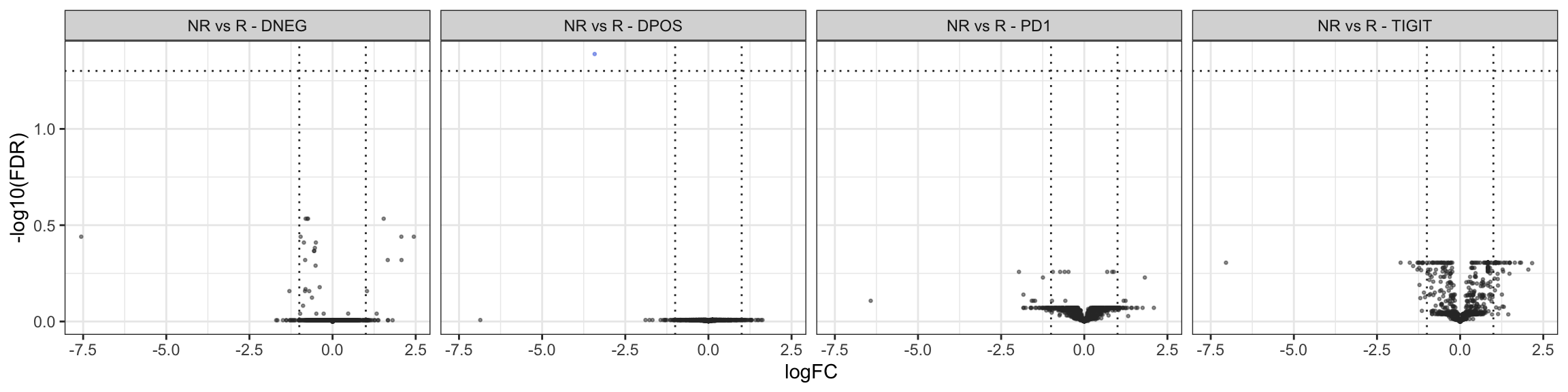
We subset the whole dataset into different subsets depending on the combination time point & treatment. An absolute log2-fold change cutoff of 1 and a false discovery rate (FDR) cutoff of 5% are used to determine differentially expressed genes (DEGs); whereas a false discovery rate (FDR) cutoff of 5% is used to determine differentially expressed gene sets (GSEA).

1.1.1 Time point T0 - DEGs

###--- DE Analysis
countData <- readRDS(file = here("output", "RNA_count.rds"))
#- Subsetting
countData.tmp <- countData[, which(countData$time.point == "T0")]
#- phenoData
phenoData.tmp <- pData(countData.tmp)
phenoData.tmp$group <- paste(phenoData.tmp$fraction, phenoData.tmp$outcome, sep = "_")
phenoData.tmp %>% View("pData")
#- Normalization factor
norm.tmp <- calcNormFactors(countData.tmp)
#- Design matrix
myDesign.tmp <- model.matrix(~ 0 + group, data = phenoData.tmp)
colnames(myDesign.tmp) <- str_remove(string = colnames(myDesign.tmp), pattern = "group")
#- Contrast matrix
aovCon.tmp <- makeContrasts(NR_vs_R_DNEG = (DNEG_NR - DNEG_R),
                            NR_vs_R_DPOS = (DPOS_NR - DPOS_R),
                            NR_vs_R_PD1 = (PD1_NR - PD1_R),
                            NR_vs_R_TIGIT = (TIGIT_NR - TIGIT_R),
                            levels = myDesign.tmp)
#- Voom transformation
voomData.tmp <- voom(counts = countData.tmp, design = myDesign.tmp, lib.size = colSums(exprs(countData.tmp)) * norm.tmp)
normData_1 <- voomData.tmp$E

###--- Fitting
fit1.tmp <- lmFit(object = voomData.tmp, design = myDesign.tmp)
fit2.tmp <- contrasts.fit(fit = fit1.tmp, contrasts = aovCon.tmp)
fit2.tmp <- eBayes(fit = fit2.tmp, trend = FALSE)

registerDoMC(2)
results_DEGs_1 <- foreach(i = 1:ncol(aovCon.tmp)) %dopar%
{
  results.tmp <- topTable(fit = fit2.tmp, adjust.method = "fdr", coef = i, number = nrow(voomData.tmp), sort = "P")
  results.tmp <- data.table(Gene = rownames(results.tmp), results.tmp)
  write_csv(x = results.tmp, path = here("output", "output_2019-02-22/", paste0("DEGs_T0_", colnames(aovCon.tmp)[i], ".csv")))
  results.tmp[, Direction := ifelse(adj.P.Val < 0.05 & sign(logFC) == 1 & abs(logFC) >= 1, "Up",
                                    ifelse(adj.P.Val < 0.05 & sign(logFC) == -1 & abs(logFC) >= 1, "Down", "NotDE"))]
  return(results.tmp)
}
names(results_DEGs_1) <- colnames(aovCon.tmp)

results_DEGs_1$NR_vs_R_DNEG[Direction != "NotDE"] # 0 DEG
results_DEGs_1$NR_vs_R_DPOS[Direction != "NotDE"] # 1 DEG
results_DEGs_1$NR_vs_R_PD1[Direction != "NotDE"] # 0 DEG
results_DEGs_1$NR_vs_R_TIGIT[Direction != "NotDE"] # 0 DEG

There are (FDR 5% & log2-FC > 1)

NR vs R - PD-1-TIGIT- - 0 DEG;
NR vs R - PD-1+TIGIT+ - 1 DEG;
NR vs R - PD-1+ - 0 DEG;
NR vs R - TIGIT+ - 0 DEG.

Volcano plots

Tables

Boxplot

1.1.2 Time point T0 - GSEA

Three databases are used (from http://software.broadinstitute.org/gsea/msigdb/collections.jsp)

KEGG pathways;
Hallmark pathways;
Immunologic signatures - c7.

###--- GSEA
gene.sets <- readRDS(file = here("data", "gene-sets", "genesets_human.rds"))
countData <- readRDS(file = here("output", "RNA_count.rds"))

#- countData & norm
countData.tmp <- countData[, which(countData$time.point == "T0")]
phenoData.tmp <- pData(countData.tmp)
phenoData.tmp$group <- paste(phenoData.tmp$fraction, phenoData.tmp$outcome, sep = "_")
norm.tmp <- calcNormFactors(countData.tmp)
myDesign.tmp <- model.matrix(~ 0 + group, data = phenoData.tmp)
colnames(myDesign.tmp) <- str_remove(string = colnames(myDesign.tmp), pattern = "group")
aovCon.tmp <- makeContrasts(NR_vs_R_DNEG = (DNEG_NR - DNEG_R),
                            NR_vs_R_DPOS = (DPOS_NR - DPOS_R),
                            NR_vs_R_PD1 = (PD1_NR - PD1_R),
                            NR_vs_R_TIGIT = (TIGIT_NR - TIGIT_R),
                            levels = myDesign.tmp)
voomData.tmp <- voom(counts = countData.tmp, design = myDesign.tmp, lib.size = colSums(exprs(countData.tmp)) * norm.tmp)

#- Get indices
registerDoMC(2)
indices.list <- foreach(i = 1:length(gene.sets)) %dopar%
{
  indices.tmp <- limma::ids2indices(gene.sets[[i]], rownames(normData_1))
  indices.tmp <- indices.tmp[sapply(indices.tmp, length) >= 5]
  return(indices.tmp)
}
names(indices.list) <- names(gene.sets)

#- GSEA - camera
registerDoMC(2)
results.GSEA_1 <- foreach(i = 1:length(results_DEGs_1)) %dopar%
{
  GSEA.tmp <- foreach(j = 1:length(indices.list)) %do%
  {
    results.tmp <- camera(voomData.tmp, indices.list[[j]], design = myDesign.tmp, contrast = aovCon.tmp[, i], sort = TRUE)
    results.tmp <- data.table(`Gene set` = rownames(results.tmp), results.tmp)
    results.tmp[, Genes := paste(rownames(voomData.tmp)[unlist(indices.list[[j]][`Gene set`])], collapse = ", "), by = `Gene set`]
    write_csv(x = results.tmp, path = here("output", "output_2019-02-22/", paste0("GSEA_T0_", names(indices.list)[j], "_", colnames(aovCon.tmp)[i], ".csv")))
    results.tmp <- results.tmp[FDR < 0.05]
    return(results.tmp)
  }
  names(GSEA.tmp) <- names(indices.list)
  return(GSEA.tmp)
}
names(results.GSEA_1) <- names(results_DEGs_1)

There are (FDR 5%)

NR vs R - PD-1-TIGIT- - 1 gene set - KEGG;
NR vs R - PD-1-TIGIT- - 1 gene set - Hallmark;
NR vs R - PD-1-TIGIT- - 0 gene set - c7;
NR vs R - PD-1+TIGIT+ - 0 gene set - KEGG;
NR vs R - PD-1+TIGIT+ - 1 gene set - Hallmark;
NR vs R - PD-1+TIGIT+ - 0 gene set - c7;
NR vs R - PD-1+ - 0 gene set - KEGG;
NR vs R - PD-1+ - 1 gene set - Hallmark;
NR vs R - PD-1+ - 0 gene set - c7;
NR vs R - TIGIT+ - 1 gene set - KEGG;
NR vs R - TIGIT+ - 1 gene set - Hallmark;
NR vs R - TIGIT+ - 0 gene set - c7.

Please look at files (results) in the output/output_2019-02-22/ folder.

1.1.3 Time point M1 - DEGs

###--- DE Analysis
countData <- readRDS(file = here("output", "RNA_count.rds"))
#- Subsetting
countData.tmp <- countData[, which(countData$time.point == "M1")]
#- phenoData
phenoData.tmp <- pData(countData.tmp)
phenoData.tmp$group <- paste(phenoData.tmp$fraction, phenoData.tmp$outcome, sep = "_")
phenoData.tmp %>% View("pData")
#- Normalization factor
norm.tmp <- calcNormFactors(countData.tmp)
#- Design matrix
myDesign.tmp <- model.matrix(~ 0 + group, data = phenoData.tmp)
colnames(myDesign.tmp) <- str_remove(string = colnames(myDesign.tmp), pattern = "group")
#- Contrast matrix
aovCon.tmp <- makeContrasts(NR_vs_R_DNEG = (DNEG_NR - DNEG_R),
                            NR_vs_R_DPOS = (DPOS_NR - DPOS_R),
                            NR_vs_R_PD1 = (PD1_NR - PD1_R),
                            NR_vs_R_TIGIT = (TIGIT_NR - TIGIT_R),
                            levels = myDesign.tmp)
#- Voom transformation
voomData.tmp <- voom(counts = countData.tmp, design = myDesign.tmp, lib.size = colSums(exprs(countData.tmp)) * norm.tmp)
normData_2 <- voomData.tmp$E

###--- Fitting
fit1.tmp <- lmFit(object = voomData.tmp, design = myDesign.tmp)
fit2.tmp <- contrasts.fit(fit = fit1.tmp, contrasts = aovCon.tmp)
fit2.tmp <- eBayes(fit = fit2.tmp, trend = FALSE)

registerDoMC(2)
results_DEGs_2 <- foreach(i = 1:ncol(aovCon.tmp)) %dopar%
{
  results.tmp <- topTable(fit = fit2.tmp, adjust.method = "fdr", coef = i, number = nrow(voomData.tmp), sort = "P")
  results.tmp <- data.table(Gene = rownames(results.tmp), results.tmp)
  write_csv(x = results.tmp, path = here("output", "output_2019-02-22/", paste0("DEGs_M1_", colnames(aovCon.tmp)[i], ".csv")))
  results.tmp[, Direction := ifelse(adj.P.Val < 0.05 & sign(logFC) == 1 & abs(logFC) >= 1, "Up",
                                    ifelse(adj.P.Val < 0.05 & sign(logFC) == -1 & abs(logFC) >= 1, "Down", "NotDE"))]
  return(results.tmp)
}
names(results_DEGs_2) <- colnames(aovCon.tmp)

results_DEGs_2$NR_vs_R_DNEG[Direction != "NotDE"] # 0 DEG
results_DEGs_2$NR_vs_R_DPOS[Direction != "NotDE"] # 0 DEG
results_DEGs_2$NR_vs_R_PD1[Direction != "NotDE"] # 0 DEG
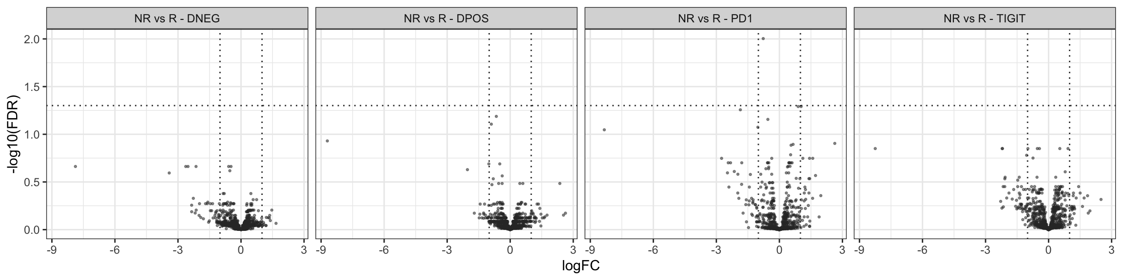
results_DEGs_2$NR_vs_R_TIGIT[Direction != "NotDE"] # 0 DEG

There are (FDR 5% & log2-FC > 1)

NR vs R - PD-1-TIGIT- - 0 DEG;
NR vs R - PD-1+TIGIT+ - 0 DEG;
NR vs R - PD-1+ - 0 DEG;
NR vs R - TIGIT+ - 0 DEG.

Volcano plots

Tables

1.1.4 Time point M1 - GSEA

Three databases are used (from http://software.broadinstitute.org/gsea/msigdb/collections.jsp)

KEGG pathways;
Hallmark pathways;
Immunologic signatures - c7.

###--- GSEA
gene.sets <- readRDS(file = here("data", "gene-sets", "genesets_human.rds"))
countData <- readRDS(file = here("output", "RNA_count.rds"))

#- countData & norm
countData.tmp <- countData[, which(countData$time.point == "M1")]
phenoData.tmp <- pData(countData.tmp)
phenoData.tmp$group <- paste(phenoData.tmp$fraction, phenoData.tmp$outcome, sep = "_")
norm.tmp <- calcNormFactors(countData.tmp)
myDesign.tmp <- model.matrix(~ 0 + group, data = phenoData.tmp)
colnames(myDesign.tmp) <- str_remove(string = colnames(myDesign.tmp), pattern = "group")
aovCon.tmp <- makeContrasts(NR_vs_R_DNEG = (DNEG_NR - DNEG_R),
                            NR_vs_R_DPOS = (DPOS_NR - DPOS_R),
                            NR_vs_R_PD1 = (PD1_NR - PD1_R),
                            NR_vs_R_TIGIT = (TIGIT_NR - TIGIT_R),
                            levels = myDesign.tmp)
voomData.tmp <- voom(counts = countData.tmp, design = myDesign.tmp, lib.size = colSums(exprs(countData.tmp)) * norm.tmp)

#- Get indices
registerDoMC(2)
indices.list <- foreach(i = 1:length(gene.sets)) %dopar%
{
  indices.tmp <- limma::ids2indices(gene.sets[[i]], rownames(normData_2))
  indices.tmp <- indices.tmp[sapply(indices.tmp, length) >= 5]
  return(indices.tmp)
}
names(indices.list) <- names(gene.sets)

#- GSEA - camera
registerDoMC(2)
results.GSEA_2 <- foreach(i = 1:length(results_DEGs_2)) %dopar%
{
  GSEA.tmp <- foreach(j = 1:length(indices.list)) %do%
  {
    results.tmp <- camera(voomData.tmp, indices.list[[j]], design = myDesign.tmp, contrast = aovCon.tmp[, i], sort = TRUE)
    results.tmp <- data.table(`Gene set` = rownames(results.tmp), results.tmp)
    results.tmp[, Genes := paste(rownames(voomData.tmp)[unlist(indices.list[[j]][`Gene set`])], collapse = ", "), by = `Gene set`]
    write_csv(x = results.tmp, path = here("output", "output_2019-02-22/", paste0("GSEA_M1_", names(indices.list)[j], "_", colnames(aovCon.tmp)[i], ".csv")))
    results.tmp <- results.tmp[FDR < 0.05]
    return(results.tmp)
  }
  names(GSEA.tmp) <- names(indices.list)
  return(GSEA.tmp)
}
names(results.GSEA_2) <- names(results_DEGs_2)

There are (FDR 5%)

NR vs R - PD-1-TIGIT- - 0 gene set - KEGG;
NR vs R - PD-1-TIGIT- - 3 gene sets - Hallmark;
NR vs R - PD-1-TIGIT- - 14 gene sets - c7;
NR vs R - PD-1+TIGIT+ - 1 gene set - KEGG;
NR vs R - PD-1+TIGIT+ - 3 gene sets - Hallmark;
NR vs R - PD-1+TIGIT+ - 41 gene sets - c7;
NR vs R - PD-1+ - 4 gene sets - KEGG;
NR vs R - PD-1+ - 0 gene set - Hallmark;
NR vs R - PD-1+ - 0 gene set - c7;
NR vs R - TIGIT+ - 1 gene set - KEGG;
NR vs R - TIGIT+ - 0 gene set - Hallmark;
NR vs R - TIGIT+ - 3 gene sets - c7.

Please look at files (results) in the output/output_2019-02-22/ folder.

1.1.5 Time point M2 - DEGs

###--- DE Analysis
countData <- readRDS(file = here("output", "RNA_count.rds"))
#- Subsetting
countData.tmp <- countData[, which(countData$time.point == "M2")]
#- phenoData
phenoData.tmp <- pData(countData.tmp)
phenoData.tmp$group <- paste(phenoData.tmp$fraction, phenoData.tmp$outcome, sep = "_")
phenoData.tmp %>% View("pData")
#- Normalization factor
norm.tmp <- calcNormFactors(countData.tmp)
#- Design matrix
myDesign.tmp <- model.matrix(~ 0 + group, data = phenoData.tmp)
colnames(myDesign.tmp) <- str_remove(string = colnames(myDesign.tmp), pattern = "group")
#- Contrast matrix
aovCon.tmp <- makeContrasts(NR_vs_R_DNEG = (DNEG_NR - DNEG_R),
                            NR_vs_R_DPOS = (DPOS_NR - DPOS_R),
                            NR_vs_R_PD1 = (PD1_NR - PD1_R),
                            NR_vs_R_TIGIT = (TIGIT_NR - TIGIT_R),
                            levels = myDesign.tmp)
#- Voom transformation
voomData.tmp <- voom(counts = countData.tmp, design = myDesign.tmp, lib.size = colSums(exprs(countData.tmp)) * norm.tmp)
normData_3 <- voomData.tmp$E

###--- Fitting
fit1.tmp <- lmFit(object = voomData.tmp, design = myDesign.tmp)
fit2.tmp <- contrasts.fit(fit = fit1.tmp, contrasts = aovCon.tmp)
fit2.tmp <- eBayes(fit = fit2.tmp, trend = FALSE)

registerDoMC(2)
results_DEGs_3 <- foreach(i = 1:ncol(aovCon.tmp)) %dopar%
{
  results.tmp <- topTable(fit = fit2.tmp, adjust.method = "fdr", coef = i, number = nrow(voomData.tmp), sort = "P")
  results.tmp <- data.table(Gene = rownames(results.tmp), results.tmp)
  write_csv(x = results.tmp, path = here("output", "output_2019-02-22/", paste0("DEGs_M2_", colnames(aovCon.tmp)[i], ".csv")))
  results.tmp[, Direction := ifelse(adj.P.Val < 0.05 & sign(logFC) == 1 & abs(logFC) >= 1, "Up",
                                    ifelse(adj.P.Val < 0.05 & sign(logFC) == -1 & abs(logFC) >= 1, "Down", "NotDE"))]
  return(results.tmp)
}
names(results_DEGs_3) <- colnames(aovCon.tmp)

results_DEGs_3$NR_vs_R_DNEG[Direction != "NotDE"] # 0 DEG
results_DEGs_3$NR_vs_R_DPOS[Direction != "NotDE"] # 0 DEG
results_DEGs_3$NR_vs_R_PD1[Direction != "NotDE"] # 0 DEG
results_DEGs_3$NR_vs_R_TIGIT[Direction != "NotDE"] # 0 DEG

There are (FDR 5% & log2-FC > 1)

NR vs R - PD-1-TIGIT- - 0 DEG;
NR vs R - PD-1+TIGIT+ - 0 DEG;
NR vs R - PD-1+ - 0 DEG;
NR vs R - TIGIT+ - 0 DEG.

Volcano plots

Tables

1.1.6 Time point M2 - GSEA

Three databases are used (from http://software.broadinstitute.org/gsea/msigdb/collections.jsp)

KEGG pathways;
Hallmark pathways;
Immunologic signatures - c7.

###--- GSEA
gene.sets <- readRDS(file = here("data", "gene-sets", "genesets_human.rds"))
countData <- readRDS(file = here("output", "RNA_count.rds"))

#- countData & norm
countData.tmp <- countData[, which(countData$time.point == "M2")]
phenoData.tmp <- pData(countData.tmp)
phenoData.tmp$group <- paste(phenoData.tmp$fraction, phenoData.tmp$outcome, sep = "_")
norm.tmp <- calcNormFactors(countData.tmp)
myDesign.tmp <- model.matrix(~ 0 + group, data = phenoData.tmp)
colnames(myDesign.tmp) <- str_remove(string = colnames(myDesign.tmp), pattern = "group")
aovCon.tmp <- makeContrasts(NR_vs_R_DNEG = (DNEG_NR - DNEG_R),
                            NR_vs_R_DPOS = (DPOS_NR - DPOS_R),
                            NR_vs_R_PD1 = (PD1_NR - PD1_R),
                            NR_vs_R_TIGIT = (TIGIT_NR - TIGIT_R),
                            levels = myDesign.tmp)
voomData.tmp <- voom(counts = countData.tmp, design = myDesign.tmp, lib.size = colSums(exprs(countData.tmp)) * norm.tmp)

#- Get indices
registerDoMC(2)
indices.list <- foreach(i = 1:length(gene.sets)) %dopar%
{
  indices.tmp <- limma::ids2indices(gene.sets[[i]], rownames(normData_3))
  indices.tmp <- indices.tmp[sapply(indices.tmp, length) >= 5]
  return(indices.tmp)
}
names(indices.list) <- names(gene.sets)

#- GSEA - camera
registerDoMC(2)
results.GSEA_3 <- foreach(i = 1:length(results_DEGs_3)) %dopar%
{
  GSEA.tmp <- foreach(j = 1:length(indices.list)) %do%
  {
    results.tmp <- camera(voomData.tmp, indices.list[[j]], design = myDesign.tmp, contrast = aovCon.tmp[, i], sort = TRUE)
    results.tmp <- data.table(`Gene set` = rownames(results.tmp), results.tmp)
    results.tmp[, Genes := paste(rownames(voomData.tmp)[unlist(indices.list[[j]][`Gene set`])], collapse = ", "), by = `Gene set`]
    write_csv(x = results.tmp, path = here("output", "output_2019-02-22/", paste0("GSEA_M2_", names(indices.list)[j], "_", colnames(aovCon.tmp)[i], ".csv")))
    results.tmp <- results.tmp[FDR < 0.05]
    return(results.tmp)
  }
  names(GSEA.tmp) <- names(indices.list)
  return(GSEA.tmp)
}
names(results.GSEA_3) <- names(results_DEGs_3)

There are (FDR 5%)

NR vs R - PD-1-TIGIT- - 5 gene sets - KEGG;
NR vs R - PD-1-TIGIT- - 3 gene sets - Hallmark;
NR vs R - PD-1-TIGIT- - 0 gene set - c7;
NR vs R - PD-1+TIGIT+ - 4 gene sets - KEGG;
NR vs R - PD-1+TIGIT+ - 3 gene sets - Hallmark;
NR vs R - PD-1+TIGIT+ - 0 gene set - c7;
NR vs R - PD-1+ - 4 gene sets - KEGG;
NR vs R - PD-1+ - 2 gene sets - Hallmark;
NR vs R - PD-1+ - 0 gene sets - c7;
NR vs R - TIGIT+ - 4 gene sets - KEGG;
NR vs R - TIGIT+ - 1 gene set - Hallmark;
NR vs R - TIGIT+ - 4 gene sets - c7.

Please look at files (results) in the output/output_2019-02-22/ folder.

sessionInfo()

R version 3.6.2 (2019-12-12)
Platform: x86_64-apple-darwin15.6.0 (64-bit)
Running under: macOS Mojave 10.14.6

Matrix products: default
BLAS:   /Library/Frameworks/R.framework/Versions/3.6/Resources/lib/libRblas.0.dylib
LAPACK: /Library/Frameworks/R.framework/Versions/3.6/Resources/lib/libRlapack.dylib

locale:
[1] fr_FR.UTF-8/fr_FR.UTF-8/fr_FR.UTF-8/C/fr_FR.UTF-8/fr_FR.UTF-8

attached base packages:
[1] grid      parallel  stats     graphics  grDevices utils     datasets 
[8] methods   base     

other attached packages:
 [1] ComplexHeatmap_2.2.0 DT_0.11              doMC_1.3.6          
 [4] iterators_1.0.12     foreach_1.4.7        here_0.1            
 [7] edgeR_3.28.0         limma_3.42.0         Biobase_2.46.0      
[10] BiocGenerics_0.32.0  data.table_1.12.8    janitor_1.2.0       
[13] forcats_0.4.0        stringr_1.4.0        dplyr_0.8.3         
[16] purrr_0.3.3          readr_1.3.1          tidyr_1.0.0         
[19] tibble_2.1.3         ggplot2_3.2.1        tidyverse_1.3.0     

loaded via a namespace (and not attached):
 [1] nlme_3.1-143        fs_1.3.1            lubridate_1.7.4    
 [4] RColorBrewer_1.1-2  httr_1.4.1          rprojroot_1.3-2    
 [7] tools_3.6.2         backports_1.1.5     R6_2.4.1           
[10] DBI_1.1.0           lazyeval_0.2.2      colorspace_1.4-1   
[13] GetoptLong_0.1.8    withr_2.1.2         tidyselect_0.2.5   
[16] compiler_3.6.2      git2r_0.26.1        cli_2.0.1          
[19] rvest_0.3.5         xml2_1.2.2          labeling_0.3       
[22] scales_1.1.0        digest_0.6.23       rmarkdown_2.0      
[25] pkgconfig_2.0.3     htmltools_0.4.0     fastmap_1.0.1      
[28] dbplyr_1.4.2        htmlwidgets_1.5.1   rlang_0.4.2        
[31] GlobalOptions_0.1.1 readxl_1.3.1        rstudioapi_0.10    
[34] shiny_1.4.0         shape_1.4.4         generics_0.0.2     
[37] farver_2.0.2        jsonlite_1.6        crosstalk_1.0.0    
[40] magrittr_1.5        Rcpp_1.0.3          munsell_0.5.0      
[43] fansi_0.4.1         lifecycle_0.1.0     stringi_1.4.5      
[46] whisker_0.4         yaml_2.2.0          promises_1.1.0     
[49] crayon_1.3.4        lattice_0.20-38     haven_2.2.0        
[52] circlize_0.4.8      hms_0.5.3           locfit_1.5-9.1     
[55] zeallot_0.1.0       knitr_1.26          pillar_1.4.3       
[58] rjson_0.2.20        codetools_0.2-16    reprex_0.3.0       
[61] glue_1.3.1          evaluate_0.14       modelr_0.1.5       
[64] png_0.1-7           vctrs_0.2.1         httpuv_1.5.2       
[67] cellranger_1.1.0    gtable_0.3.0        clue_0.3-57        
[70] assertthat_0.2.1    xfun_0.12           mime_0.8           
[73] xtable_1.8-4        broom_0.5.3         later_1.0.0        
[76] workflowr_1.6.0     cluster_2.1.0

- RNA-seq - DE Analysis (3) -

1 Statistical Analysis

1.1 Differential analysis btw outcomes within each time point

1.1.1 Time point T0 - DEGs

1.1.2 Time point T0 - GSEA

1.1.3 Time point M1 - DEGs

1.1.4 Time point M1 - GSEA

1.1.5 Time point M2 - DEGs

1.1.6 Time point M2 - GSEA